- A data structure is a logical way that data is organized
- Uses:
- Decision making
- Numerical and statistical analysis
- Blockchain
RAM
- Each integer takes 4 bytes. Each character takes 1 byte.
- Each byte is 8 bits
- Array store values at contiguous memory locations
Arrays
Static arrays
- Contiguous block of data
- Index starts at 0
- Static arrays are fixed sized arrays (not really a concern of Python or JavaScript)
- We delete values by overwriting, such as with a 0
- Static array operations: - Reading /writing at i-th position: - Insert / remove at end: - Insert / remove middle:
Dynamic arrays
- Pushing / popping at the end:
- After dynamic array increases in size and takes new spot in memory, old array is deallocated. The amoritized time complexity of pushing to a dynamic array is . because we are going to be runnig out of space infrequently (on average).
- Time complexities same as static arrays.
Stacks
- Linear data structure, LIFO (Last In First Out)
- Uses:
- Temporary storage during recursive operations
- Redo and undo operations in doc editors
- Reversing a string
- Parenthesis matching
- Postfix to Infix expressions
- Function calls order
- Stack methods:
- push
- pop
- top
- isEmpty
- size
Queue
- Linear data structure, items are added to the rear end. Items are removed from the front of the queue.
- Uses:
- Breadth-first search algorithm in graphs
- Operating systems: job scheduling, disk scheduling, CPU scheduling
- Methods:
- enqueue
- dequeue
- isEmpty
- rear
- front
- size
Doubly ended queue (deque)
- Deques allow items to be inserted at either end
- Types of deques:
- Input restricted deques: insertion operations are performed at only one end while deletion is performed at both ends
- Output restricted deque: deletion operations are performed at only one end while insertion is performed at both ends in the output restricted queue
- Methods:
- insertFront(): This adds an element to the front of the Deque.
- insertLast(): This adds an element to the rear of the Deque.
- deleteFront(): This deletes an element from the front of the Deque.
- deleteLast():This deletes an element from the front of the Deque.
- getFront(): This gets an element from the front of the Deque.
- getRear(): This gets an element from the rear of the Deque.
- isEmpty(): This checks whether Deque is empty or not.
- isFull(): This checks whether Deque is full or not.
Priority queue
- Each element is assigned a priority value
- The order in which elements in a priority queue are served is determined by their priority
- Uses:
- Used in graph algorithms like Dijkstra, Prim’s Minimum spanning tree etc.
- Huffman code for data compression
- Finding Kth Largest/Smallest element
- Different implementations
| Operations | peek | insert | delete |
|---|---|---|---|
| Linked List | O(1) | O(n) | O(1) |
| Binary Heap | O(1) | O(log n) | O(log n) |
| Binary Search Tree | O(1) | O(log n) | O(log n) |
Difference between stack and queue
| Stack | Queue |
|---|---|
| Stack is a linear data structure where data is added and removed from the top. | Queue is a linear data structure where data is ended at the rear end and removed from the front. |
| Stack is based on LIFO (Last In First Out) principle | Queue is based on FIFO (First In First Out) principle |
| Insertion operation in Stack is known as push. | Insertion operation in Queue is known as enqueue. |
| Delete operation in Stack is known as pop. | Delete operation in Queue is known as dequeue. |
| Only one pointer is available for both addition and deletion: top() | Two pointers are available for addition and deletion: front() and rear() |
| Used in solving recursion problems | Used in solving sequential processing problems |
Arrays
- One-dimensional array: stores elements in contiguous memory locations, accessing them using a single index value. It is a linear data structure holding all the elements in a sequence
- Two-dimensional array: tabular array that includes rows adn columns and stores data. An two-dimensional array is created by grouping rows and columns.
Linked List
- A series of linked nodes (or items) that are connected by links. Each link represents an entry into the linekd list, and each entry points to the next node in the sequence. The order in which nodes are added to the list is determined by the order in which they are created.
- Uses
- Stack, queue, binary trees, and graphs are implemented using linked lists
- Dynamic management for oeprating system memory
- Round robin scheduling for operating system tasks
- Forward and backward operation in the browser
- Difference between array and linked list
Arrays Linked Lists An array is a collection of data elements of the same type. A linked list is a collection of entities known as nodes. The node is divided into two sections: data and address. It keeps the data elements in a single memory. It stores elements at random, or anywhere in the memory. The memory size of an array is fixed and cannot be changed during runtime. The memory size of a linked list is allocated during runtime. An array's elements are not dependent on one another. Linked List elements are dependent on one another. It is easier and faster to access an element in an array. In the linked list, it takes time to access an element. Memory utilization is ineffective in the case of an array. Memory utilization is effective in the case of linked lists. Operations like insertion and deletion take longer time in an array. Operations like insertion and deletion are faster in the linked list.
Hash Sets / Maps
-
Hash maps don’t maintain orders
-
Cannot contain duplicates, just like a BST or TreeMap
-
Average time complexities
- Insert:
- Remove:
- Search:
-
A hashtable is a collection of key value pairs
-
Each key value pair is known as an entry
-
Each storage location is a bucket
-
Common resolution for a collision in a linked list: turn each bucket into a linked list
-
Methods
getandputhave complexity assuming the hash function used in the hash map distributes elements uniformly among the buckets -
The key or value object that gets used in the hashmap must implement these methods:
equals()used when trying to retrieve a value from the maphashcode()method is used when inserting the key object into the map
-
When hashmap is half full, its size is doubled. When it is doubled, it needs to be rehashed (elements need to be placed into correct positions)
-
Hash map implementation
names = ["alice", "brad", "collin", "brad", "dylan", "kim"]

countMap = {}

for name in names:
     if name not in countMap:
          countMap[name] = 1;
     else:
          countMap[name] += 1;
const names = ["alice", "brad", "collin", "brad", "dylan", "kim"]; const countMap = new Map(); for (let i = 0; i < names.length; i++) { // If countMap does not contain name if (!countMap.has(names[i])) { countMap.set(names[i], 1); } else { countMap.set(names[i], countMap.get(names[i]) + 1); } }
Binary trees
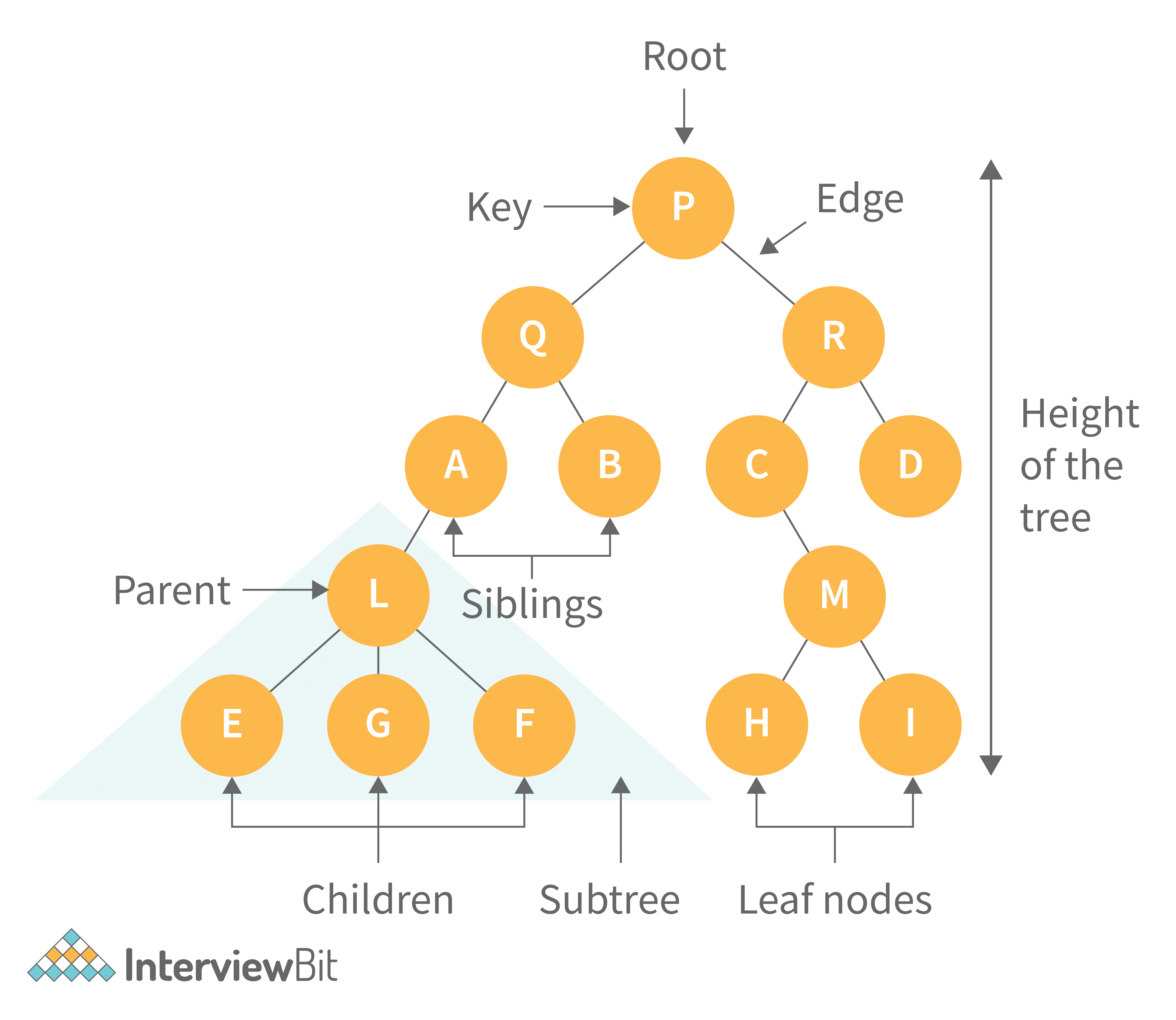
Binary search tree
- All elements in the left subtree of a node should have a value less than or equal to the parent node’s value
- All elements in the right subtree of a node should have a value greater than or equal to the parent node’s value
- Insertion in balanced BST takes time
Depth First Search
class TreeNode {
  constructor(val) {
    this.val = val;
    this.left = null;
    this.right = null;
  }
}

/*
1. travel to the left most node
2. process it
3. check if it has any right subtrees
4. if yes, process that
5. then pop back up one level, process it, then process its subtree

time complexity: O(n), same as sorted array
*/

// processes in ascending order
function inorder(root) {
  if (root == null) {
    return;
  }
  inorder(root.left);
  console.log(root.val);
  inorder(root.right);
}

// process a node before moving on to its children
function preorder(root) {
  if (root == null) {
    return;
  }
  console.log(root.val);
  preorder(root.left);
  preorder(root.right);
}

// process the left and right subtree, and then process root node
function postorder(root) {
  if (root == null) {
    return;
  }
  postorder(root.left);
  postorder(root.right);
  console.log(root.val);
}
Breadth first search
class TreeNode {
  constructor(val) {
    this.val = val;
    this.left = null;
    this.right = null;
  }
}

function bfs(root) {
  let queue = [];
  if (root != null) {
    queue.push(root);
  }
  let level = 0;
  while (queue.length > 0) {
    console.log("level " + level + ": ");
    let levelLength = queue.length;
    for (let i = 0; i < levelLength; i++) {
      let curr = queue.shift();
      console.log(curr.val + " ");
      if (curr.left != null) {
        queue.push(curr.left);
      }
      if (curr.right != null) {
        queue.push(curr.right);
      }
    }
    level++;
    console.log();
  }
}
Tree traversal
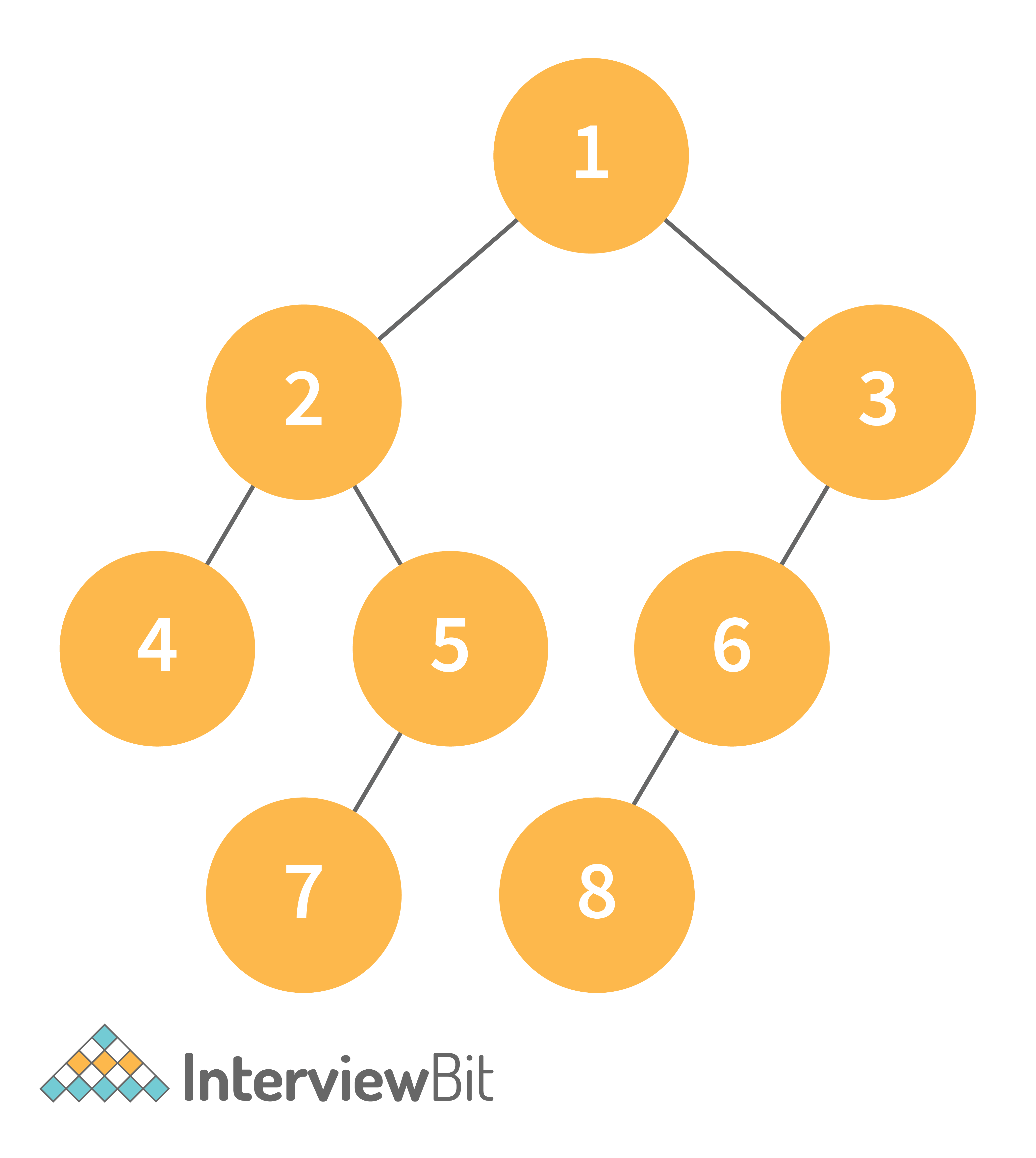
- Inorder Traversal => Left, Root, Right : [4, 2, 5, 1, 3]
- Preorder Traversal => Root, Left, Right : [1, 2, 4, 5, 3]
- Postorder Traversal => Left, Right, Root : [4, 5, 2, 3, 1]
Inorder traversal
- In binary search trees, inorder traversal gives nodes in ascending order
- Algorithm:
- Traverse the left subtree
- Visit the root.
- Traverse the right subtree
Preorder traversal
- Preorder traversal is commonly used to create a copy of the tree
- It is also used to get prefix expression of an expression tree
- Algorithm:
- Visit the root
- Traverse the left subtree
- Traverse the right subtree
Postorder traversal
- Postorder traversal is commonly used to delete the tree
- It is also used to get the postfix expression of an expression tree
- Algorithm:
- Traverse the left subtree
- Traverse the right subtree
- Visit the root
Graph
-
Non-linear data structure made up of nodes and edges
-
The nodes are also known as vertices, and edges are lines or arcs that connect two nodes
-
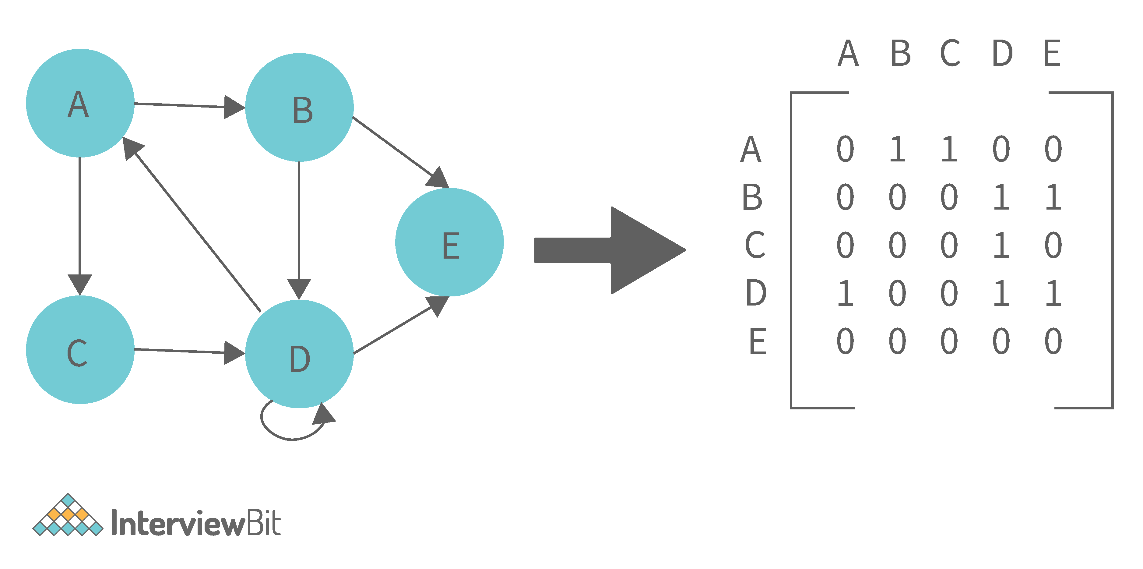
Two most common graph representations:
-
Adjacency matrix: two-dimensional array with the dimensions , where is the number of vertices in a graph. It takes time to remove an edge. Queries such as whether there is an edge from vertex to vertex are efficient and can be done in O(V^2)O(V)$ time.
-
Adjacency list: each node holds a list of nodes that are directly connected to that vertex. In the worst case, a graph can have edges, consuming space. It is simpler to add a vertex, and it takes the least amount of time to compute all of a vertex’s neighbors. In the worst case, checking adjacency takes time in the worst case.
-
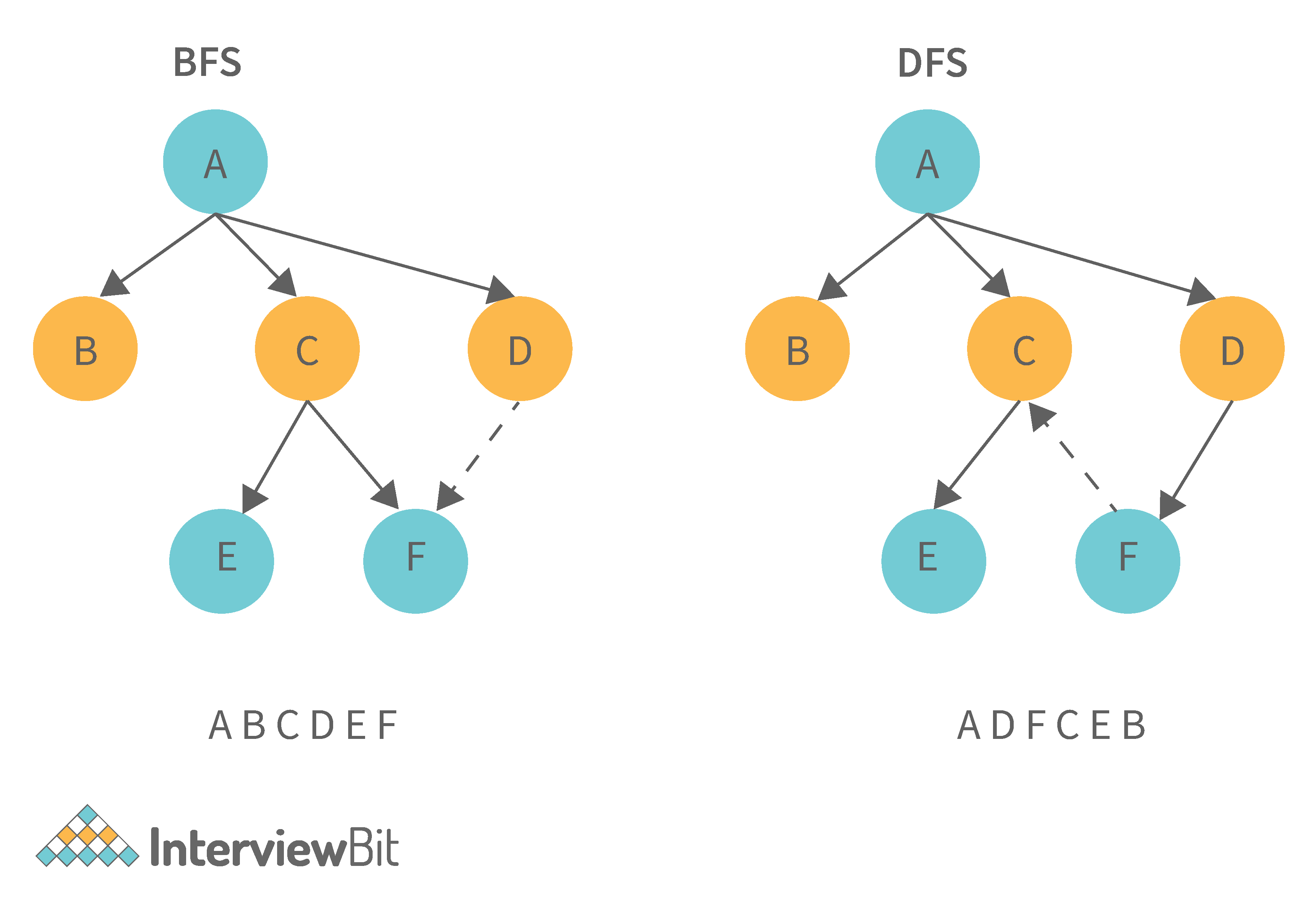
Breadth First Search (BFS) and Depth First Search (DFS)
| Breadth First Search (BFS) | Depth First Search (DFS) |
|---|---|
| It stands for “Breadth First Search” | It stands for “Depth First Search” |
| BFS (Breadth First Search) finds the shortest path using the Queue data structure. | DFS (Depth First Search) finds the shortest path using the Stack data structure. |
| We walk through all nodes on the same level before passing to the next level in BFS. | DFS begins at the root node and proceeds as far as possible through the nodes until we reach the node with no unvisited nearby nodes. |
| When compared to DFS, BFS is slower. | When compared to BFS, DFS is faster. |
| BFS performs better when the target is close to the source. | DFS performs better when the target is far from the source. |
| BFS necessitates more memory. | DFS necessitates less memory. |
| Nodes that have been traversed multiple times are removed from the queue. | When there are no more nodes to visit, the visited nodes are added to the stack and then removed. |
| Backtracking is not an option in BFS. | The DFS algorithm is a recursive algorithm that employs the concept of backtracking. |
| It is based on the FIFO principle (First In First Out). | It is based on the LIFO principle (Last In First Out). |
AVL Tree
- Height balancing binary search trees
- Compares the heights of the left and right subtrees and ensures that the difference is less than one. This is called the balance factor:
- Methods: same as binary search tree, but rotations are performed to balance
the tree
- Insertion
- Deletion
- Four types of rotations:
- Left rotation: When a node is inserted into the right subtree of the right subtree and the tree becomes unbalanced, we perform a single left rotation.
- Right rotation: If a node is inserted in the left subtree of the left subtree, the AVL tree may become unbalanced. The tree then requires right rotation.
- Left-Right rotation: The RR rotation is performed first on the subtree, followed by the LL rotation on the entire tree.
- Right-Left rotation: The LL rotation is performed first on the subtree, followed by the RR rotation on the entire tree.
- Uses:
- AVL trees are typically used for in-memory sets and dictionaries.
- AVL trees are also widely used in database applications where there are fewer insertions and deletions but frequent data lookups are required.
- Apart from database applications, it is used in applications that require improved searching.
B-Tree
- B-Tree is a type of m-way tree that is commonly used for disc access.
- A B-Tree with order m can onlu have m-1 keys and m children.
- One of the primary reasons for using a B-Tree is its ability to store a large number of keys in a single node as well as large key values while keeping the tree’s height relatively small
- Properties:
- All of the leaves are at the same height.
- The term minimum degree ‘t’ describes a B-Tree. The value of t is determined by the size of the disc block.
- Except for root, every node must have at least t-1 keys. The root must contain at least one key.
- All nodes (including root) can have no more than 2*t - 1 keys.
- The number of children of a node is equal to its key count plus one.
- A node’s keys are sorted in ascending order. The child of two keys k1 and k2 contains all keys between k1 and k2.
- In contrast to Binary Search Tree, B-Tree grows and shrinks from the root.
- Uses:
- It is used to access data stored on discs in large databases.
- Using a B tree, you can search for data in a data set in significantly less time.
- The indexing feature allows for multilevel indexing.
- The B-tree approach is also used by the majority of servers.
Red-black tree
- Self-balancing binary tree
- Each node is either red or black. By comparing the node colors on any simple path from the root to a leaf, red-black trees ensure that no path is more than twice as long as any other, ensuring that the tree is generally balanced
- Red-black trees are similar binary trees in that they both store their data in two’s complementary binary formats
- Red-black trees are faster to access than binary trees
- Properties:
- Every node is either red or black.
- The tree’s root is always black.
- There are no two red nodes that are adjacent.
- There is the same number of black nodes on every path from a node to any of its descendant’s NULL nodes.
- All of the leaf nodes are black.
Tree Maze
Backtracking
Example problem: Determine if a path exists from the root of the tree to a leaf node. It may not contain any zeros
- The idea is to check every possibility, and backtrack if the solution fails
- If the solution fails, we return false
- That’s how the root node would know that the solution failed
- If the recursion returns true, we found a solution
function canReachLeaf(root) {
  if (root == null || root.val == 0) {
    return false;
  }
  if (root.left == null && root.right == null) {
    return true;
  }
  if (canReachLeaf(root.left)) {
    return true;
  }
  if (canReachLeaf(root.right)) {
    return true;
  }
  return false;
}
Modified problem: return the path as well
function leafPath(root, path) {
  if (root == null || root.val == 0) {
    return false;
  }
  path.push(root.val);
  if (root.left == null && root.right == null) {
    return true;
  }
  if (leafPath(root.left, path)) {
    return true;
  }
  if (leafPath(root.right, path)) {
    return true;
  }
  path.pop();
  return false;
}
Heap / Priority Queue
- Heap is implemented with a complete binary tree, could be a minheap or a maxheap
- Adding and popping takes time
- Distinction: Binary tree, NOT a binary search tree
- Order property:
- In min heap, root is smaller than every single descendant
- This is true recursively
- Reverse is true for max heap
- Tree is implemented using arrays, index starting at 1
- leftChild: 2*i
- rightChild: 2*i + 1
- parent: i/2 (round down when using a right child)
- Structure property:
- All levels are completely filled except possibly the last level
- The last level has all elements as left as possible
- Max heap
- In a Max-Heap the data element present at the root node must be the greatest among all the data elements present in the tree.
- This property should be recursively true for all sub-trees of that binary tree.
- Min heap
- In a Min-Heap the data element present at the root node must be the smallest (or minimum) among all the data elements present in the tree.
- This property should be recursively true for all sub-trees of that binary tree.
Push / Pop
Push
- To push, insert at the end of the array
- Swap with parent until order property is satisfied
- Time complexity: height of the tree, , where n is the number of nodes
Pop
- To remove the root, replace it with the last value of the tree (array)
- Swap with child until order property is satisfied
- Algorithm
// If size == 1, heap is empty, return null
// If size == 2, heap just has the root value, pop and return
// Assign the root, result = heap[1], to a temp variable
// Assign last value in array to root
// Percolate down while we at least have a left child
// Case 1: Two children
// Case 2: Just a left child
// Case 3: No children
Heapify
- Process of building a heap
- algorithm
Graphs
- Non-linear data structure made up of nodes (vertices) and edges (pointers)
- Node can be pointing to itself
- Types of graphs:
- Directed graph: edges have a direction
- Undirected graph: edges do not have a direction
- Weighted graph: edges have a weight
- Unweighted graph: edges do not have a weight
- Three kinds:
- Matrix (common)
- Typically a square matrix
- 0 or 1 values represent if a path exists
- The 2D array is the graph space itself
- Adjacency matrix (less common)
- Typically a square matrix
- Each index represents an edge between a node / vertex
- ajacencyMatrix[i][j] = 1 if there is an edge from i to j
- ajacencyMatrix[j][i] = 1 if there is an edge from i to j
- Space complexity:
- Adjacency list (most common)
- Neighbors list of each node contains a list of all the nodes it is connected to / pointing to
- Matrix (common)
Graph algorithms
Matrix DFS
Time complexity: Memory complexity:
// Count paths (backtracking)
function dfs(grid, r, c, visit) {
    let ROWS = grid.length, COLS = grid[0].length;

    if (Math.min(r, c) < 0 || r == ROWS || c == COLS ||
        visit[r][c] == 1 || grid[r][c] == 1) {
        return 0;
    }
    if (r == ROWS - 1 && c == COLS - 1) {
        return 1;
    }
    visit[r][c] = 1;

    let count = 0;
    count += dfs(grid, r + 1, c, visit);
    count += dfs(grid, r - 1, c, visit);
    count += dfs(grid, r, c + 1, visit);
    count += dfs(grid, r, c - 1, visit);

    visit[r][c] = 0;
    return count;
}

print dfs((grid, 0, 0, [][]));
Matrix BFS
Time and memory complexity:
// Matrix (2D Grid)
let grid = [
  [0, 0, 0, 0],
  [1, 1, 0, 0],
  [0, 0, 0, 1],
  [0, 1, 0, 0],
];

// Shortest path from top left to bottom right
function bfs(grid) {
  let ROWS = grid.length;
  let COLS = grid[0].length;
  let visit = new Array(4).fill(0).map(() => Array(4).fill(0)); // 4x4 2d array
  let queue = new Array();

  queue.push(new Array(2).fill(0)); // Add {0, 0}
  visit[0][0] = 1;

  let length = 0;
  while (queue.length > 0) {
    let queueLength = queue.length;
    for (let i = 0; i < queueLength; i++) {
      let pair = queue.shift();
      let r = pair[0],
        c = pair[1];

      if (r == ROWS - 1 && c == COLS - 1) {
        return length;
      }
      // We can directly build the four neighbors
      let neighbors = [
        [r, c + 1],
        [r, c - 1],
        [r + 1, c],
        [r - 1, c],
      ];
      for (let j = 0; j < 4; j++) {
        let newR = neighbors[j][0],
          newC = neighbors[j][1];
        if (
          Math.min(newR, newC) < 0 ||
          newR == ROWS ||
          newC == COLS ||
          visit[newR][newC] == 1 ||
          grid[newR][newC] == 1
        ) {
          continue;
        }
        queue.push(neighbors[j]);
        visit[newR][newC] = 1;
      }
    }
    length++;
  }
  return length; // This should never be called
}
Adjacency List
// GraphNode used for adjacency list
class GraphNode {
  constructor(val) {
    this.val = val;
    this.neighbors = new Array();
  }
}

function buildAdjList() {
  let adjList = new Map();
  let edges = [
    ["A", "B"],
    ["B", "C"],
    ["B", "E"],
    ["C", "E"],
    ["E", "D"],
  ];
  adjList.set("A", new Array());
  adjList.set("B", new Array());

  for (let edge of edges) {
    let src = edge[0],
      dst = edge[1];
    if (!adjList.has(src)) {
      adjList.set(src, new Array());
    }
    if (!adjList.has(dst)) {
      adjList.set(dst, new Array());
    }
    adjList.get(src).push(dst);
  }
  return adjList;
}

// Count paths (backtracking)
function dfs(node, target, adjList, visit) {
  if (visit.has(node)) {
    return 0;
  }
  if (node == target) {
    return 1;
  }
  let count = 0;
  visit = new Set();
  visit.add(node);
  for (let neighbor of adjList.get(node)) {
    count += dfs(neighbor, target, adjList, visit);
  }
  visit.delete(node);
  return count;
}

// Shortest path from node to target.
function bfs(node, target, adjList) {
  let length = 0;
  let visit = new Set();
  let q = [];
  visit.add(node);
  q.push(node);

  while (q.length != 0) {
    let queueLength = q.length;

    for (let i = 0; i < queueLength; i++) {
      let curr = q.shift();
      if (curr === target) {
        return length;
      }
      for (let neighbor of adjList.get(curr)) {
        if (!visit.has(neighbor)) {
          visit.add(neighbor);
          q.push(neighbor);
        }
      }
    }
    length++;
  }
  return length;
}